If you split a local LLM across multiple devices, you will lose speed. That’s been the rule since the first RPC layer-split experiment: cut the model in half across two GPUs and you lose half your tokens per second. Push it over WiFi and you lose even more.
We ran an overnight session to find the exact shape of that cliff — and somewhere between the last measurement and this one, the cliff disappeared.
The testbed
Three machines, four inference devices, everything cross-checked with repeated runs:
- Desktop: 2× Intel Arc Pro B70 32GB (Ryzen 7 5700X3D, 64GB)
- Laptop A: Intel Core Ultra 9 285H with Arc 140T iGPU (WiFi)
- Laptop B: i5-12450H with UHD Xe-LP iGPU (WiFi) — added mid-session, with a custom Windows build of Cascadia against OpenVINO 2026.5 beta1
- Model: Qwen3.8-27B INT4 (OpenVINO IR) — a hybrid: 48 DeltaNet linear-attention layers + 16 full-attention layers
Sixteen benchmark configurations later, every number below is a median of 3–5 streaming runs at batch 1.
The result that shouldn’t be possible
Same machine, two GPUs, model split 32 layers / 32 layers:
| Config | Decode speed | Retained |
|---|---|---|
| Single Arc Pro B70 | 23.78 tok/s | 100% |
| Two B70s, Cascadia pipeline | 24.02 tok/s | 101% |
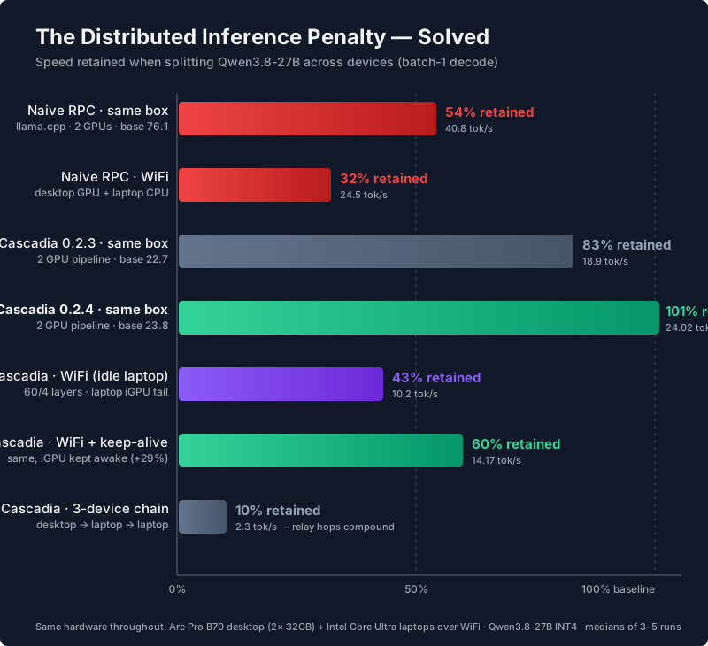
The pipeline is as fast as doing everything on one GPU. Measured relay cost: 0.249 ms per frame median. For comparison, llama.cpp RPC on the same two cards retained 54% (76.1 → 40.8 tok/s) — and the previous Cascadia build retained 83% (18.9 tok/s from a 22.7 base).
This isn’t a trick of the baseline: the single-GPU number was re-measured on the same binary, the same night. What changed is upstream engineering — between cascadia 0.2.3 and 0.2.4 the pipeline’s per-token overhead effectively vanished. A second GPU is now pure profit: 64GB of pooled VRAM serving a 27B model at full single-card speed, with prefill at parity too (1.98s vs 1.87s first-token latency on a 2,100-token prompt).
What actually kills distributed inference (it’s not the network)
The WiFi experiments tell the real story. Adding a laptop as the tail stage of the pipeline, over WiFi:
| Layers on the laptop | Decode speed |
|---|---|
| 32 of 64 | 7.0 tok/s |
| 16 of 64 | 8.9 tok/s |
| 8 of 64 | 10.1 tok/s |
| 4 of 64 | 10.2 tok/s |
The curve plateaus — because the per-frame wire cost is only 2.6 ms (measured, p50). The network was never the bottleneck. The bottleneck is a fixed ~45–55 ms per-token cost on the laptop stage: the 636MB language-model head lands on the tail device, and — the fun part — the iGPU falls asleep between tokens.
The +29% fix: don’t let the GPU sleep
We noticed decode ran 37% faster immediately after a long prefill — the only difference was that the iGPU was still awake. So we ran the intervention: a 30-line Python script doing one tiny matmul on the laptop’s iGPU every 50 ms while the pipeline decodes.
- Idle tail: 10.49 tok/s (noisy: 9.9–10.5)
- With keep-alive: 14.17 tok/s (dead stable: 13.9–14.2 across runs)
That’s +29–35% from power management alone, replicated at two keep-alive intervals. The best WiFi configuration now retains 60% of single-GPU speed — while serving layers the desktop never had to compute. This should be a worker feature (an idle-loop warmup between relay frames), and the variance collapse tells you the laptop’s power states were also the source of the run-to-run noise.
When pooling devices wins (and when it doesn’t)
The honest negative results matter as much:
- Deep chains lose. Three devices in a row (desktop → laptop → laptop): 2.3 tok/s. Four stages: 1.95 tok/s. Every extra relay hop adds ~70 ms of wake-and-queue latency per token — worse than the compute you offload.
- Slow iGPUs don’t pay. The Xe-LP laptop as a 16-layer tail: 4.6 tok/s, roughly half of what the 140T manages on the identical split.
- Single-stream kernels still rule. vLLM on one B70 does 106.7 tok/s — 4.5× Cascadia’s best single-stream number. Different game; Cascadia’s edge is orchestration, not kernels.
So the playbook we measured:
- Second GPU, same machine → pipeline it: free capacity, zero speed loss (101%).
- Throughput for concurrent users → run independent servers per GPU: we measured 47.8 tok/s aggregate from two single-GPU instances with zero interference — double what any pipeline of the same hardware achieves.
- Laptops over WiFi → only as capacity relief, only with few layers (≤8), and keep the GPU awake.
Why this time is different
Every number here decomposes into a latency model that predicts all 14 configurations within ~10%: 0.6 ms/layer on the B70s, ~2.3 ms/layer on the 140T, the language-model head’s cost on whatever device owns the last layer, 2.6 ms/frame on WiFi, ~70 ms per relay hop, and a now-quantified power-management penalty. When a distributed system’s losses are explained by measured constants instead of hand-waving, you can finally engineer them away — one of them (the relay overhead) was already engineered to zero upstream, and another (the sleeping tail) fell to a 30-line script.
The benchmark data lives on the intelinside.ai leaderboards, and the engine patches that make heterogeneous pipelines tunable (--ov-* flag passthrough, custom layer splits) are headed upstream to Cascadia.