Chapter 4 LLM Handbook Part 4: Quantization & the KL-Divergence Budget

Why quantize at all?

A 27B-parameter model stored in FP16 needs $27 \times 10^9 \times 2 \approx 54$ GB — far more than a 32 GB GPU. Quantization shrinks each weight from 16 bits (or 32) down to 4–8 bits so the model fits. The trade: every weight becomes slightly wrong, and those small errors accumulate into a slightly different output distribution.

The engineering question is not “is quantization lossless?” (it never is). It is: for a fixed VRAM budget, which quantization loses the least quality?

What quantization does to a weight

Quantization snaps a continuous range of values onto a small set of discrete levels. INT4 has 16 levels; INT8 has 256. The gap between a true value and its nearest level is the rounding error.

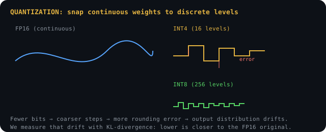
Two things make the error worse:

• Fewer bits → coarser steps → bigger rounding error.
• Outliers → a few huge weights stretch the range, making every other step coarser. This is why “K-quants” (Q4_K, Q5_K, Q6_K) group weights into blocks and give the important blocks more bits.

Measuring the damage: KL-divergence

We can’t just eyeball quality. Instead we compare the model’s output probability distribution before and after quantization. KL-divergence (Kullback–Leibler) measures how much one distribution differs from another:

$$D_{KL}(P ,|, Q) = \sum_x P(x) \log \frac{P(x)}{Q(x)}$$

where $P$ is the FP16 (reference) distribution and $Q$ is the quantized one. $D_{KL}=0$ means identical. In practice:

KL-divergence	Feel
< 0.01	Near-lossless; hard to spot
0.01 – 0.05	Minor degradation on edge cases
0.05 – 0.5	Noticeable; reasoning suffers
> 1	Broken; output incoherent

The KV cache is quantization too

The same idea applies to the KV cache (Part 1). But here there is an asymmetry that matters enormously:

• Keys (K) decide which tokens to attend to. Quantizing K badly changes the routing → catastrophic.
• Values (V) are averaged across attended tokens. Quantizing V is mostly harmless.

Measured on real hardware, quantizing K to q40 gives $D{KL} \approx 5.5$ (broken), while keeping K at q80 and compressing only V to q4_1 gives $D{KL} \approx 0.003$ (near-lossless) at ~50% of the FP16 KV memory:

K cache	V cache	KL-div	Verdict
q8_0	q4_1	~0.003	Fleet standard
q5_0	q4_1	~0.008	Acceptable
q4_0	any	~5.5	Never

Rule of thumb: spend your bits on K, save them on V. Never drop K below 8 bits.

Spending a fixed VRAM budget

Given $B$ bytes of VRAM, you choose a three-way split: weights, KV cache (context), and compute buffers. Lower weight quant frees bytes for more context; but too-low weight quant raises KL. The optimum is usually:

• Weights at Q4_K–Q6_K (near-lossless for most models),
• KV at q8_0 K + q4_1 V,
• Whatever context length the remainder buys.

This is exactly the budgeting done for the Intel Arc Pro B70 32GB in the companion case studies — see the b70 category for the measured results.

Where to go next

• Part 5 (planned): Memory bandwidth — why decode speed is bytes/second, and why MoE models decode faster.
• Part 6 (planned): Speculative decoding & MTP — amortizing the bandwidth cost.